
Hi, This is my first article about Machine Learning and Artificial Intelligence which I would like to share regarding to my knowledge and experience. In this article we are going to focus on ML first, so let’s get started.
Source code of this article can be download from GitHub right here.
In general Machine Learning model can be classified into 3 categories.
The first one is “Supervised Learning Algorithms” which is require 2 types of data set. Input data set(input data set) and an answered data set (output data set) in order to let learning algorithms learn and explore relationship among them. For example input data set can be set of car images in many aspect for each model/brand while output data set are labeled classes of those images regarding to their model or brand.
The second kind of model called “Un-Supervised Learning Algorithms” which only input data set are required. Then learning algorithms are going to learn pattern of input data itself.
Third kind of machine learning is “Reinforcement learning” which consider how intelligent agents ought to take actions in an environment in order to maximize the notion of cumulative reward. Reinforcement learning is one of three basic machine learning paradigms, alongside supervised learning and unsupervised learning.
Let’s take a look at Supervised Learning Algorithms first. Normally there are several learning algorithms such as Perceptron, Logistic Regression, SVM etc.
1. Supervised Learning Algorithms
1.1 Perceptron Linear-Classifier
from sklearn import datasets
from sklearn.model_selection import train_test_split
from sklearn.preprocessing import StandardScaler
from sklearn.linear_model import Perceptron
from sklearn.metrics import accuracy_score
from matplotlib.colors import ListedColormap
from matplotlib.axes._axes import _log as matplotlib_axes_logger
matplotlib_axes_logger.setLevel('ERROR')
%matplotlib inline

import matplotlib.pyplot as plt
import numpy as np
import numpy as np
iris = datasets.load_iris()
X = iris.data[:, [2,3]]
y = iris.target
X_train, X_test, y_train, y_test = train_test_split(X, y, test_size=0.3, random_state=0)
sc = StandardScaler()
sc.fit(X_train)
X_train_std = sc.transform(X_train)
X_test_std = sc.transform(X_test)
ppn = Perceptron(max_iter=40, tol=1e-3, eta0=0.1, random_state=0)
ppn.fit(X_train_std, y_train)
y_pred = ppn.predict(X_test_std)
print('Misclassified samples: %d' % (y_test != y_pred).sum())
print('Accuracy: %.2f' % accuracy_score(y_test, y_pred))
And the result is

def plot_decision_regions(X, y, classifier,
    test_idx=None, resolution=0.02):

    markers = ('s', 'x', 'o', '^', 'v')
    colors = ('red', 'blue', 'lightgreen', 'gray', 'cyan')
    cmap = ListedColormap(colors[:len(np.unique(y))])

    x1_min, x1_max = X[:, 0].min() - 1, X[:, 0].max() + 1
    x2_min, x2_max = X[:, 1].min() - 1, X[:, 1].max() + 1
    xx1, xx2 = np.meshgrid(np.arange(x1_min, x1_max, resolution),
    np.arange(x2_min, x2_max, resolution))
    Z = classifier.predict(np.array([xx1.ravel(), xx2.ravel()]).T)
    Z = Z.reshape(xx1.shape)
    plt.contourf(xx1, xx2, Z, alpha=0.4, cmap=cmap)
    plt.xlim(xx1.min(), xx1.max())
    plt.ylim(xx2.min(), xx2.max())

    X_test, y_test = X[test_idx, :], y[test_idx]
    for idx, cl in enumerate(np.unique(y)):
        plt.scatter(x=X[y == cl, 0], y=X[y == cl, 1],
        alpha=0.8, c=cmap(idx), marker=markers[idx], label=cl)

    if test_idx:
        X_test, y_test = X[test_idx, :], y[test_idx]
        plt.scatter(X_test[:, 0], X_test[:, 1], c='',
            alpha=1.0, linewidth=1, marker='o', s=55, label='test set')

X_combined_std = np.vstack((X_train_std, X_test_std))
y_combined = np.hstack((y_train, y_test))
plot_decision_regions(X=X_combined_std, y=y_combined, classifier=ppn, test_idx=range(105,150))
plt.xlabel('petal length [standardized]')
plt.ylabel('petal width [standardized]')
plt.legend(loc='upper left')
plt.show()
1.2 Logistic Regression
import matplotlib.pyplot as plt
import numpy as np
def sigmoid(z):
    return 1.0 / (1.0 + np.exp(-z))

z = np.arange(-7,7,0.1)
phi_z = sigmoid(z)
plt.plot(z, phi_z)
plt.axvline(0.0, color='k')
plt.axhspan(0.0, 1.0, facecolor='1.0', alpha=1.0, ls='dotted')
plt.axhline(y=0.5, ls='dotted', color='k')
plt.yticks([0.0, 0.5, 1.0])
plt.ylim(-0.1, 1.1)
plt.xlabel('z')
plt.ylabel('$\phi (z)$')
plt.show()
from sklearn.linear_model import LogisticRegression

lr = LogisticRegression(C=1000.0, random_state=0, solver="lbfgs", multi_class="auto")
lr.fit(X_train_std, y_train)
plot_decision_regions(X_combined_std, y_combined, classifier=lr, test_idx=range(105,150))
plt.xlabel('petal length [standardized]')
plt.ylabel('petal width [standardized]')
plt.legend(loc='upper left')
plt.show()
print("Classes",lr.classes_)
lr.predict_proba(X_test_std)

1.3 Support Vector Machines
from sklearn.svm import SVC
svm = SVC(kernel='linear', C=1.0, random_state=0)
svm.fit(X_train_std, y_train)
plot_decision_regions(X_combined_std,
y_combined, classifier=svm,
test_idx=range(105,150))
plt.xlabel('petal length [standardized]')
plt.ylabel('petal width [standardized]')
plt.legend(loc='upper left')
plt.show()
Logistic regression vs SVM
In general classification tasks, Logistic Regression and SVM provide the same results. However because Logistic Regression try to maximize conditional likelihoods from training data set, therefore it more sensitive to outliers than SVM. While SVM mostly care about data set’s points that are closet to the decision boundary (Support Vectors).
By the way Logistic Regression still have some advantage for example it is more simpler model compare to SVM and also fit for streaming data.
1.4 Solving “Nonlinear” problems using a kernel SVM
Another reason why SVM gained more popularity in ML applications is that they can be easily kernelized to solve non-linear classification problems. One example of non-linear classification problem is XOR gate problem.
np.random.seed(0)
X_xor = np.random.randn(50, 2)
y_xor = np.logical_xor(X_xor[:, 0] > 0, X_xor[:, 1] > 0)
y_xor = np.where(y_xor, 1, -1)
plt.scatter(X_xor[y_xor==1, 0], X_xor[y_xor==1, 1],
c='b', marker='x', label='1')
plt.scatter(X_xor[y_xor==-1, 0], X_xor[y_xor==-1, 1],
c='r', marker='s', label='-1')
plt.ylim(-3.0)
plt.legend()
plt.show()
positions = X_xor
groups = y_xor
svm = SVC(kernel='rbf', random_state=0, gamma=0.1, C=10.0)
svm.fit(positions, groups)
plot_decision_regions(positions, groups, classifier=svm)
plt.legend(loc='upper left')
plt.show()
gamma = 0.1 is cut-off parameter of Gaussian sphere. If we increase gamma’s value it will increase data set’s influence as well which will lead to softer decision boundary.
Here are example of how to apply RBF (Radial Basis Function) kernel to SVM in order to classify Iris data set.
svm = SVC(kernel='rbf', random_state=0, gamma=0.2, C=1.0)
svm.fit(X_train_std, y_train)
plot_decision_regions(X_combined_std,y_combined, classifier=svm, test_idx=range(105,150))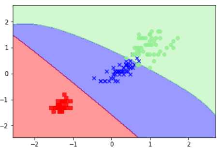
svm = SVC(kernel='rbf', random_state=0, gamma=1.0, C=1.0)
svm.fit(X_train_std, y_train)
plot_decision_regions(X_combined_std,
y_combined, classifier=svm,
test_idx=range(105,150))
plt.xlabel('petal length [standardized]')
plt.ylabel('petal width [standardized]')
plt.legend(loc='upper left')
plt.show()
svm = SVC(kernel='rbf', random_state=1, gamma=10.0, C=1.0)
svm.fit(X_train_std, y_train)
plot_decision_regions(X_combined_std,
y_combined, classifier=svm,
test_idx=range(105,150))
plt.xlabel('petal length [standardized]')
plt.ylabel('petal width [standardized]')
plt.legend(loc='upper left')
plt.show()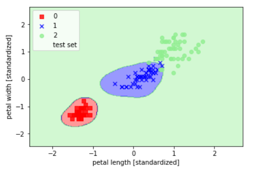
1.5 Decision Tree Learning
Build Decision Tree
Decision Tree able to generate complex decision boundaries by divide features spaces in rectangular shape. We can create multi-layer depth decision tree but we have to beware over fitting as well. In my case I set maximum depth = 3
from sklearn.tree import DecisionTreeClassifier
tree = DecisionTreeClassifier(criterion='entropy', max_depth=3, random_state=0)
tree.fit(X_train, y_train)
X_combined = np.vstack((X_train, X_test))
y_combined = np.hstack((y_train, y_test))
plot_decision_regions(X_combined, y_combined,
classifier=tree, test_idx=range(105,150))
plt.xlabel('petal length [cm]')
plt.ylabel('petal width [cm]')
plt.legend(loc='upper left')
plt.show()
1.6 Random Forests
Random Forests also gained popularity among ML applications due to it’s good classification performance, scalability and ease to use. Conceptually Random Forests are combination of decision trees called “Ensemble Learning” which are combine weak learners in order to build robust model or strong learner. Random Forests algorithms finally create more accurate and less over fitting model.
Random Forests have 4 learning steps
- Create n random bootstrap (randomly pick n samples from training data set with replacement).
- Grow Decision Trees from those bootstrap samples, in each node:
- Randomly pick d features without replacement.
- Split node by using features whose provide the best split result according to Objective Function e.g maximize information gain.
3. Repeat step 1 and 2 k times.
4. Aggregate prediction results from each tree in order to assign classes label by using majority vote method.
from sklearn.ensemble import RandomForestClassifier
forest = RandomForestClassifier(criterion='entropy',
n_estimators=10,
random_state=1,
n_jobs=7)
forest.fit(X_train, y_train)
plot_decision_regions(X_combined, y_combined,
classifier=forest, test_idx=range(105,150))
plt.xlabel('petal length')
plt.ylabel('petal width')
plt.legend(loc='upper left')
plt.show()
1.7 K-nearest neighbors
K-nearest neighbors differ from previous learning algorithms in term of it’s not a learning discriminative function but “Remember training data set” instead.
Parametric vs Non-parametric models
Machine Learning algorithms can be classified into 2 categories which are “Parametric” and “Non-Parametric” model.
Parametric model: Is parameters estimation based model. This kind of model learn and estimate parameters from training data set in order to create ML model that can classify new data set without requiring the original training data set any more.
Non-Parametric model: In contrast this kind of model cannot be characterized by a fixed set of parameters, and number of parameters also grows with the training data as well e.g Decision Tree Classifier/Random Forests and Kernel SVM model.
KNN belongs to Non-Parametric model class called “Instance-based learning model” this kind of model always remember training data set.
KNN have 3 learning steps
- Choose k and distance metric values.
- Find closet k data points for classification process.
- Assign class label by using majority vote method.
The main advantage of this memory-based model is that the classifier immediately adapts as we collect new training data. However the main disadvantage is computational complexity issue which will grows linearly side by side with the number of samples data set. In order to reduce computational complexity issue Dimensionality Reduction (e.g LSA, SVD) or Features Selection techniques must be applied to data set before feed to the model.
from sklearn.neighbors import KNeighborsClassifier
knn = KNeighborsClassifier(n_neighbors=100, p=1, metric='minkowski')
knn.fit(X_train_std, y_train)
plot_decision_regions(X_combined_std, y_combined,
classifier=knn, test_idx=range(105,150))
plt.xlabel('petal length [standardized]')
plt.ylabel('petal width [standardized]')
plt.show()
1.8 Dimensionality Reduction
Here is example of how to apply Singular Value Decomposition (SVD) to documents classification tasks
from numpy import zeros
from scipy.linalg import svd
from matplotlib import pyplot as plt
from matplotlib import cm as CM
from matplotlib import colors
import numpy as np
%matplotlib inline
from math import log
from numpy import asarray, sum
titles = ["10 Best Places to Visit in Spain – Touropia Travel Experts",
          "9 Tips for Traveling in Japan | Fodor's Travel",
          "Places to Visit in Italy | Where to go in Italy | Rough Guides",
          "First Time to Japan 10 Travel Tips to Plan Your Trip. | The Shooting Star",
          "Japan Travel Guide | Fodor's Travel",
"The Neatest Little Guide to Stock Market Investing",
"Investing For Dummies, 4th Edition",
"The Little Book of Common Sense Investing: The Only Way to Guarantee Your Fair Share of Stock Market Returns"]

stopwords = ["and","edition","for","in","little","of","the","to"]
ignorechars = ''',:'!'''
class LSA(object):

    def __init__(self, stopwords, ignorechars):
        self.stopwords = stopwords
        self.ignorechars = ignorechars
        self.wdict = {}
        self.dcount = 0

    def parse(self, doc):
        words = doc.split();
        for w in words:
            w = w.lower().translate(self.ignorechars)
            if w in self.stopwords:
                continue
            elif w in self.wdict:
                self.wdict[w].append(self.dcount)
            else:
                self.wdict[w] = [self.dcount]
        self.dcount += 1

    def build(self):
        self.keys = [k for k in self.wdict.keys() if len(self.wdict[k]) > 1]
        self.keys.sort()
        self.A = zeros([len(self.keys), self.dcount])
        for i, k in enumerate(self.keys):
            for d in self.wdict[k]:
                self.A[i,d] += 1

    def calc(self):
        self.U, self.S, self.Vt = svd(self.A)

    def printA(self):
        print('Here is the count matrix')
        print(self.A)

    def printSVD(self):
        print('Here are the singular values (S)')
        print(self.S)
        print('Here are the first 3 columns of the U matrix (Words)')
        print(-1*self.U[:, 0:3])
        print('Here are the first 3 rows of the Vt matrix (Titles)** (Will be used for classification)')
        print(-1*self.Vt[0:3, :])
        print(self.Vt.shape)
        fig, ax = plt.subplots()
        heatmap = ax.pcolor(-1*self.Vt[0:3, :], cmap=plt.cm.seismic)
        cbar = plt.colorbar(heatmap)
        column_labels = ['', 'Doc1', 'Doc2', 'Doc3', 'Doc4', 'Doc5', 'Doc6','Doc7', 'Doc8', 'Doc9']
        row_labels = ['', '  Dimension1', '', '  Dimension2', '', '  Dimension3']
        ax.set_xticklabels(column_labels, minor=False)
        ax.set_yticklabels(row_labels, minor=False)
        plt.xticks(rotation=90)
        ax = plt.gca()
        plt.show()
        for i in range(0,8):
            if ((-1*self.Vt[1, i])<0) & ((-1*self.Vt[2, i])<0):
                print('Group 1 Doc: ', i,' ',titles[i])
        print("")
        for i in range(0,8):
            if ((-1*self.Vt[1, i])>0) & ((-1*self.Vt[2, i])>0):
                print('Group 2 Doc: ', i,' ',titles[i])
        print("")
        for i in range(0,8):
            if ((-1*self.Vt[1, i])<0) & ((-1*self.Vt[2, i])>0):
                print('Group 3 Doc: ', i,' ',titles[i])
        print("")
        for i in range(0,8):
            if ((-1*self.Vt[1, i])>0) & ((-1*self.Vt[2, i])<0):
                print('Group 4 Doc: ', i,' ',titles[i])
mylsa = LSA(stopwords, ignorechars)
for t in titles:
    mylsa.parse(t)

mylsa.build()
mylsa.printA()
mylsa.calc()
mylsa.printSVD()

Now we are going to take a look second kind of ML model which able to learn and find pattern or relationship among input data set itself. These kind of learning model such as K-Means Clustering, DBSCAN etc.
2. Un-Supervised Learning Algorithms
2.1 K-Means Clustering
Basically clustering algorithms can be applied to solve several business problems such as documents/music/movies classification by their topics including business users clustering by their purchase history, payment history or their profiles. K-Means Clustering is one of the building block to build recommendation engine.
from sklearn.datasets import make_blobs
import matplotlib.pyplot as plt

X, y = make_blobs(n_samples=150,
    n_features=2,
    centers=3,
    cluster_std=0.5,
    shuffle=True,
    random_state=0)

plt.scatter(X[:,0], X[:,1],c='Red',marker='o',s=50)

plt.grid()
plt.show()
Now we have data set consists of 150 data points which roughly grouped in 3 groups and visualize in 2D plane as shown above.
K-Means Clustering have 4 steps
- Randomly pick k centroids from data points called cluster’s initial centroids or seed centroids.
- Assign remain data points to the closet centroid(i).
- Re-calculate and update each centroid to the new point.
- Repeat step 2 and 3 until get stable centroid points or exceed maximum round.
from sklearn.cluster import KMeans
km = KMeans(n_clusters=4,
init='random',
n_init=10,
max_iter=300,
tol=1e-04,
random_state=0)
y_km = km.fit_predict(X)
plt.scatter(X[y_km==0,0],
    X[y_km ==0,1],
    s=50,
    c='lightgreen',
    marker='s',
    label='cluster 1')

plt.scatter(X[y_km ==1,0],
    X[y_km ==1,1],
    s=50,
    c='orange',
    marker='o',
    label='cluster 2')

plt.scatter(X[y_km ==2,0],
    X[y_km ==2,1],
    s=50,
    c='lightblue',
    marker='v',
    label='cluster 3')

plt.scatter(km.cluster_centers_[:,0],
    km.cluster_centers_[:,1],
    s=250,
    marker='*',
    c='red',
    label='centroids')

plt.legend()
plt.grid()
plt.show()
2.2 Locating regions of high density via DBSCAN
DBSCAN using local regions technique, a special label assigned to each sample (point) using the following criteria.
- Any data point will be considered as core points if they have number of neighbor data points in ε radius equal or more than (MinPts).
- Any data point will be considered as border points if they have number of neighbor data points in ε radius less than (MinPts) but lies within the ε radius of a core point ε.
- All other points that are neither core nor border points are considered as noise points.
from sklearn.datasets import make_moons

X, y = make_moons(n_samples=200,
    noise=0.05,
    random_state=0)

plt.scatter(X[:,0], X[:,1])
plt.show()
km = KMeans(n_clusters=2,
    random_state=0)

y_km = km.fit_predict(X)

plt.scatter(X[y_km==0,0],
    X[y_km==0,1],
    c='lightblue',
    marker='o',
    s=40,
    label='cluster 1')

plt.scatter(X[y_km==1,0],
    X[y_km==1,1],
    c='red',
    marker='s',
    s=40,
    label='cluster 2')

plt.legend()
plt.show()
Main advantage of DBSCAN is it not assume that cluster radius must be circular shape like K-Means does.
from sklearn.cluster import DBSCAN

db = DBSCAN(eps=0.2,
    min_samples=5,
    metric='euclidean')

y_db = db.fit_predict(X)

plt.scatter(X[y_db==0,0],
    X[y_db==0,1],
    c='lightblue',
    marker='o',
    s=40,
    label='cluster 1')

plt.scatter(X[y_db==1,0],
    X[y_db==1,1],
    c='red',
    marker='s',
    s=40,
    label='cluster 2')

plt.legend()
plt.show()

These are most of ML algorithms I know which are covered both Supervised and Un-Supervised learning algorithms.
I hope this article helpful to you and next time I going to share more in A.I related topics for example Artificial Neural Networks, Quantum Computing and so on, Thank you.